A survey of Object Detection: The R-CNN series
Introduction
In the first post of the new year (and decade!), we’re going to go over the R-CNN series - a set of incrementally improved methods that serve as the foundation for how object detection (via deep learning) is carried out today.
The papers that we’ll discuss today are:
-
Rich feature hierarchies for accurate object detection and semantic segmentation [1]
-
Fast R-CNN [2]
-
Faster R-CNN - Towards Real-Time Object Detection with Region Proposal Networks [3]
Brief introduction to object detection as a problem
Object detection, as a problem, is the combination of localization and classification; the goal is to identify objects in an image, draw accurate bounding boxes around them and classify the bounded objects as a particular class.
To measure how good or bad an object detector is, we usually use a metric called the mAP (Mean average precision); given a set of predictions, ranked by confidence, we calculate a running precision (how accurate predictions are, calculated as \(\frac{\text{TP}}{\text{TP + FP}}\)) and recall (the ability of the model to recall positive examples, calculated as \(\frac{\text{TP}}{\text{TP + FN}}\)), and average the precision at various recall values. If you’re looking for a deeper explanation of the metric, check out this [Medium post] by Jonathan Hui!
R-CNN (Regions with CNN features)
In 2012, AlexNet [5] demonstrated the superiority of CNN based methods for image classification, outperforming traditional CV approaches. Could the same hold true for object detection too?
Yes! Published in 2014, the R-CNN paper used the advancements from AlexNet to incorporate CNNs into the object detection pipeline with great success. As shown in Figure 1, the core idea was simple - the authors replaced the feature extraction phase in Section 3, which used traditional feature extractors such as SIFT [6] and HOG [7], with AlexNet by using the vector from the penultimate fully-connected layer as the feature vector.
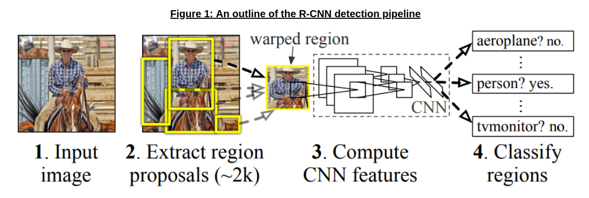
While the picture painted by Figure 1 is fairly straightforward, there are two details to fill in - how regions are proposed, and how the feature vector is used to classify.
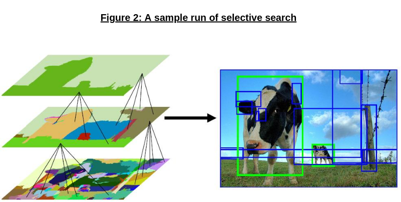
- Region proposals: Region proposal uses a mechanism known as selective search [8], although the R-CNN method itself is agnostic to how regions are proposed (as it just warps each region to a fixed size and feeds it into AlexNet). Selective search uses Felzenszwalb and Huttenlocher’s graph-based image segmentation algorithm as a starting point [9]; it then repeatedly merges the two most similar neighboring regions (in a manner similar to agglomerative clustering) to generate a new region, and repeats this until the entire image is a single region. Below in Figure 2 (from the original paper), we can see a sample run of selective search hierarchically generating region proposals, which are then converted into bounding boxes.
- Classification: Classification, given the feature vector, is done using an SVM for each class to score a proposed region; the authors also incorporate greedy non-maximum suppression, which rejects a region that has a high overlap (measured using intersection-over-union) with a higher scoring region for the same class, avoiding the issue of duplicate predictions for the same object.
Fast R-CNN
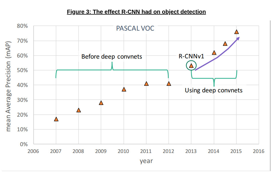
With R-CNN, object detection had begun to harness the power of deep convnets (as shown in Figure 3 courtesy Ross Girshick [10] below), achieving much better mAP scores than before.
However, there were a fair few problems with the method:
-
Multiple training objectives: The R-CNN system had three different trainable modules, each of which had their own objective/loss function:
-
The CNN was pre-trained on ImageNet image classification, and fine-tuned to classify object classes using warped proposals via a log loss/softmax objective
-
The per-class SVMs trained to do the actual test-time object classification use the hinge loss
-
The bounding box regressors (used to smoothen object proposals into well formed boxes) use a squared loss term
This inherently posed a challenge to create an end-to-end trainable system, since you could not backpropogate the loss from the SVMs or regressors to improve the CNN for the task at hand.
-
-
Slow inference: Because each proposed region was run through the CNN module separately, this led to very slow test-time inference (on the order of ~47s/image)
-
Expensive to train: The R-CNN method, as currently defined, took over 84 hours to train; this stems to a degree from the same problem of running each proposal through the CNN, but also required hundreds of gigabytes of storage for the extracted feature vectors (used to train the SVMs)
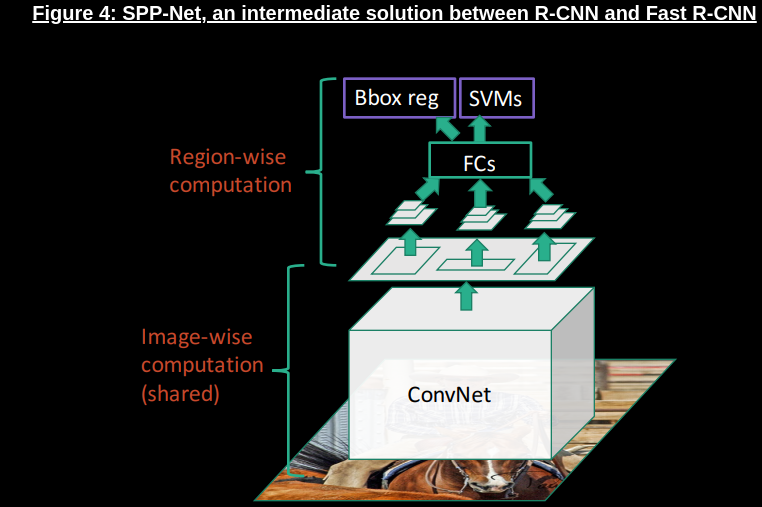
While methods like SPP-Net [11] solved some of these problems, as shown in Figure 4, some subset of these problems still existed in R-CNN based systems - until Fast R-CNN came along!
Core ideas
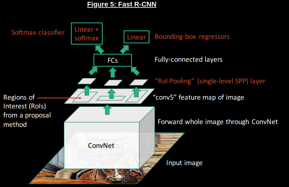
As you can see from Figure 5 above, the Fast R-CNN network looks fairly similar to SPP-Net. However, there are a few key differences:
-
No more SVMs: The first key difference is the replacement of per-class SVMs with a linear+softmax layer, along with the linearization of the bounding box regressors; this allows the network to directly use the losses from the upstream object detection task to train the convolutional modules (by backpropogating a multi-task loss), and removes the need to cache extracted feature vectors on disk, reducing the storage burden for the network.
-
ROI pooling: The second key difference is the ROI pooling layer; SPP-Net has a similar layer, but on multiple scales (extracting features at multiple scales is a common trick in computer vision), while Fast R-CNN only does this at one scale. There are two parts to this layer:
-
Projection : Since the first few layers are just convolutions (as explained well [here]), you could run these layers on a region proposal, which would be part of the feature map for the image as a whole. As shown in the diagrams for Figures 4/5, we can therefore calculate the “projection” of a ROI proposal onto the generated feature map,which allows us to use one forward pass of the image to calculate all the CNN-based features for every proposal together.
-
Pooling: The pooling mechanism itself is pretty similar to the one used in pooling layers in general CNNs; the projected ROI window is divided up into a fixed number of sub-windows/grids (allowing us to deal with arbitrarily sized proposals), and each subgrid is max pooled to generate a fixed size output for the pooling layer. The key point here is that the layer is differentiable - we can pass the gradient back into the portion of the feature maps that were “argmaxed” during pooling, allowing us to train the network almost entirely end-to-end (the “almost” becomes more relevant when we discuss Faster R-CNN in the next section)!
-
-
Hierarchical sampling: Given the emphasis on shared computation, the Fast R-CNN method also advocates using hierarchical sampling - instead of sampling a small number of regions from many different images, the authors sampled a lot of ROIs from two images! This allowed the method to effectively use the shared computation of feature maps between different ROIs for the same image, and significantly sped up training for the network as a whole.
The results for Fast R-CNN were simply amazing - the method achieved a ~9x speedup in training time over R-CNN and a 146x speedup in test-time inference, requiring only 0.32s/image - all while achieving a better mAP and requiring less disk storage.
Faster R-CNN
However, the authors weren’t done quite yet!
As we saw with Fast R-CNN, almost the entire object detection pipeline had become end-to-end, with the exception of region proposals. The R-CNN series usually used selective search, but was agnostic to the method of region proposals; while this meant you could plug in your desired method, it also meant that proposals themselves were often slow, and did not learn from the fine-tuning of the rest of the network on the dataset of choice.
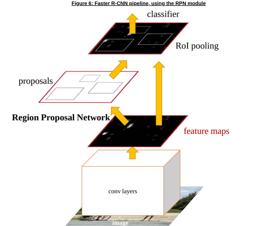
To solve this problem, the authors of Faster R-CNN came up with the Region Proposal Network (RPN), a convolutional network that generates region proposals; the RPNs, as shown in Figure 6 below, could share feature maps with the object detection pipeline, which made the proposals much more efficient and differentiable, enabling end-to-end training!
Region Proposal Networks (RPN)
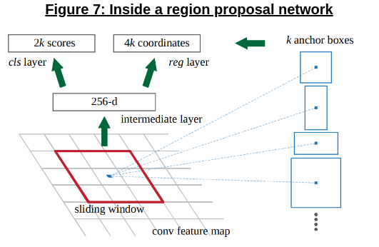
Figure 7 (above) shows us the fundamental ideas behind the RPN; given a feature map (generated from the same backbone used for ROI pooling in Fast R-CNN), the network “slides” over the feature map, generating proposals from the center of each sliding window. For each proposal, the RPN generates:
-
Scores, representing the probability of an object existing in the area of the image corresponding to the generated region.
-
4 offsets, representing the change with reference to each of the \(k\) anchor boxes that are initialized to the center of the sliding window (\(\delta x_{\text{center}}, \delta y_{\text{center}}, \delta \text{ width and } \delta \text{ height }\))
Underlying these are a few key details, as we discuss below:
-
Anchor boxes: The anchor boxes are a key part of what makes the RPN work; as shown in Figure 7, the network initializes \(k\) different anchor boxes, “anchored” to the center of the current window. These boxes, critically, are of different scales and/or aspect ratios, which allows RPN to generate a varied set of proposals for differently-sized objects; they are also translation-invariant (objects translated in an image will still have the same (effective) proposals when run through the RPN-pipeline), a desired property in computer vision.
-
Sliding window: It’s important to note that the anchor boxes and sliding windows are implicit in the design of the RPN module and how upstream layers use the output, but are not implemented directly by looping an actual window over the feature map. Instead, given an \(n \times n\) sliding window, the easiest way to implement it is by using a \(n \times n\) conv layer, following it up with two sibling \(1 \times 1\) conv layers to output the scores and offsets - upstream layers will simply correlate these with the corresponding anchors.
-
The RPN loss function: The RPN is trained directly from the ground-truth boxes for an image by treating proposals with the highest IOU to a particular ground-truth box (or an IOU above a threshold, usually 0.7) as positive samples. Given this objectness “truth” for each proposal, the RPN is then trained with a multi-task loss - a combination of a log loss on the objectness scores predicted and a smooth \(L_{1}\) regression loss between the predicted anchor and the ground truth for all positive samples.
Training Faster R-CNN
Returning to the broader picture in Figure 7, there still remains the question - how do you train the entire network end-to-end? While many strategies are possible, the authors went with a 4-stage alternating training scheme, alternating between RPN and Faster R-CNN in a clever way:
-
(1) RPN: In this stage, the authors train the RPN network directly, using the ImageNet ground-truth proposals
-
(2) Fast R-CNN: Using the proposals from (1) but not the conv weights, the authors trained a Fast R-CNN network, with a separate set of convolutional weights.
-
(3) Fine-tune RPN: At this stage, the authors share the conv weights from R-CNN, and fine-tune the RPN; however, the shared conv layers are kept fixed, and only the unique RPN layers are tuned
-
(4) Fine-tune Fast R-CNN: In similar fashion to (3), Fast R-CNN is fine-tuned keeping the shared convolutional weights with RPN fixed, only focusing on the upstream detection layers.
Results
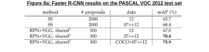
As shown in Figure 8a above, the results from Faster R-CNN were very impressive; using the RPN with a VGG backbone [13] allowed the network to do substantially better on the test set than selective search + Fast R-CNN, while generating a significantly lower number of proposals.
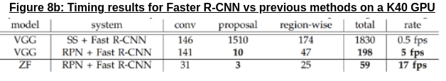
Furthermore, as shown in Figure 8b below, Faster R-CNN was also much quicker than the SS + Fast R-CNN method; this is very clearly attributed to the much quicker proposals (as shown by the timing breakdown in ms), enabling quicker detections; the fact that it could go even quicker with a different backbone (ZFNet [14]) also showed promise, as you could use smaller backbones depending on your application.
Conclusion
As we’ve seen through this article, the R-CNN series was critical in accelerating object detection throughout the mid 2010s, leveraging the power of deep learning and CNNs to slowly turn the entire pipeline into an end-to-end trainable system; the methods are still extremely powerful today, and form the foundation for many current methods in object detection.
Citations
- [1] Rich feature hierarchies for accurate object detection and semantic segmentation: Girshick et al, 2014
- [2] Fast R-CNN: Girshick et al, 2015
- [3] Faster R-CNN - Towards Real-Time Object Detection with Region Proposal Networks: Ren et al, 2016
- [4] mAP - Mean average precision for object detection: Jonathan Hui
- [5] ImageNet Classification with Deep Convolutional Neural Networks: Krizhevsky et al, 2012
- [6] Distinctive Image Features from Scale-Invariant Keypoints: Lowe, 2004
- [7] Histograms of Oriented Gradients for Human Detection: Dalal et al, 2005
- [8] Selective Search for Object Recognition: Uijlings et al, 2013
- [9] Efficient Graph-Based Image Segmentation: Felzenszwalb and Huttenlocher, 2004
- [10] Fast R-CNN talk: Ross Girshick, 2015
- [11] Spatial Pyramid Pooling in Deep Convolutional Networks for Visual Recognition: He et al, 2015
- [12] Fast RCNN: Applying ROIs to feature map: StackOverflow
- [13] Very Deep Convolutional Networks For Large-Scale Image Recognition: Simonyan et al, 2014
- [14] Visualizing and Understanding Convolutional Networks: Zeiler et Fergus, 2013