(Above: An electric transformer, that I think oddly looks like an actual Transformer network, image courtesy [1]

My first post on NLP is actually going to be split into two parts.

In today’s post (1a), we’re going to discuss the Transformer network [2] (Vaswani et al, 2017)
In the next post (1b), we’ll go over three “descendants” of the Transformer - GPT [3] (Radford et al, 2018), GPT-2[4] (Radford et al, 2019) and BERT [5] (Devlin et al, 2019).

These networks, only developed over the last 2-3 years, have quickly replaced Recurrent Neural Networks and their variants (LSTMs, GRUs) as the new state-of-the-art for all kinds of NLP based tasks, so I wanted to go deeper into these networks and understand how and why they are so effective.

I originally planned on making one post, but soon realized the material was too large and dense to cover and communicate effectively in one mega-post, so I hope you read both of them (as they come out) to get the full picture of the Transformer world!

What problem do Transformers try and solve?

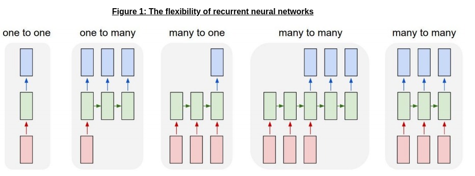
For a significant amount of time, recurrent neural networks (and variants) were the predominant models in NLP; they were extremely flexible (as shown in Figure 1 [6]), and could model longer and longer inputs well with cell structures like LSTMs and GRUs.

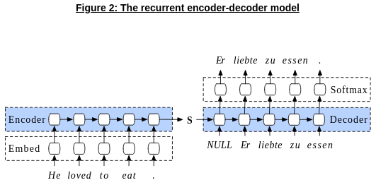
The default structure in NLP, therefore, was an encoder-decoder mechanism based on the famous Seq2Seq paper [7] in 2014 as shown by the example below in Figure 2 (courtesy Stephen Merrity [8]) :

However, in terms of training and scaling these models, there were serious issues. Predominantly, all variants of recurrent neural networks are very sequential in nature; each step of computation relies on the previous steps/states, making it hard to parallelize and scale up such models, for the following reasons:

It’s hard to vectorize/parallelize training for LSTMs; if I have a length \(n\) input sentence I want to feed into to my LSTM, I have to feed each token in one-by-one; in contrast, for instance, a CNN takes an entire image in one go!
This sequential nature of the network leads to smaller batch sizes (per GPU) due to the increased amount of computation and stored states required for training; this, in turn, also causes more memory accesses per epoch, making training more inefficient.

The problem of scale and computation is especially magnified in NLP; for instance, the Seq2Seq model by Sutskever et al has ~ 380 million parameters, and was trained on a dataset with 12 million sentences, 348 million French words and 304 million English words! Without significant parallelization capabilities, training these models is a real challenge - even if you have lots of GPUs, you need to be able to spread the load across them effectively.

To solve this problem, the authors of the Transformer network eschewed recurrence entirely in their models, replacing it with a mechanism that had already seen use alongside recurrence in NLP and other areas - attention.

Background: Attention mechanisms

Attention, as the name suggest, is a mechanism strongly inspired by human attention. To understand it better, let’s do a thought exercise.

Below is a beautiful image I pulled off the internet ([9]) - look at it, and think about your answer to the following questions.

First off - what kind of animal is in the image below?

Now, look back at the image (above) - what plant is in the image?

If you did that exercise and think about what you just did, you’ll notice something pretty interesting.

When I asked you about the bird, your eyes focused on the center of the image, and almost instantly realized it was as a bird. (If you’re an avid birdwatcher, you might have even gone further and identified it as a robin - if so, nice one!)

However, when it came to the next question, your eyes did not look (for too long) in the center; instead, they darted around the edges, until you managed to see (and identify) the sunflower.

In both cases, your mind used the context it had to attend to different parts of the input; this is the core idea of attention as a mechanism, looking for the relevant parts in an input based on your current context and state.

In the context of NLP, attention had been proposed as a method to give more context when decoding and producing the output; below, in Figure 3, we see one of the first such uses, in the seminal work Neural Machine Translation by Learning to Jointly Align and Translate by Bahdanau et al [10] in 2016.

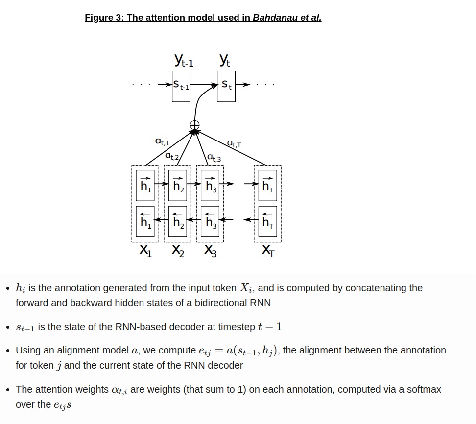
At each time step, the decoder (on top) receives a set of annotations weighted by their importance to \(y_{t}\), the word/token the decoder will output at this time step, along with the previous state, helping it pay attention to the relevant parts of the input. We can see this in Figure 4 (below), which visualizes the attention weights at different stages on an input English sentence while translating to French:

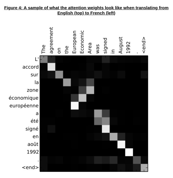
The attention weights for each generated word in French usually correspond to the word (or set of words) in English relevant to the translation; as an example, the word “zone” (in French) had strong weights on area, as opposed to the word “European” (which was the matching word to zone, from a pure sentence length perspective).

As we have seen so far, it is evident that attention can effectively encode the interactions between different parts of the input, especially in the context of a desired output; Transformer networks, however, developed the attention mechanism to a new level, allowing us to solely rely on it for both encoding and decoding inputs.

Transformers: Attention is all you need

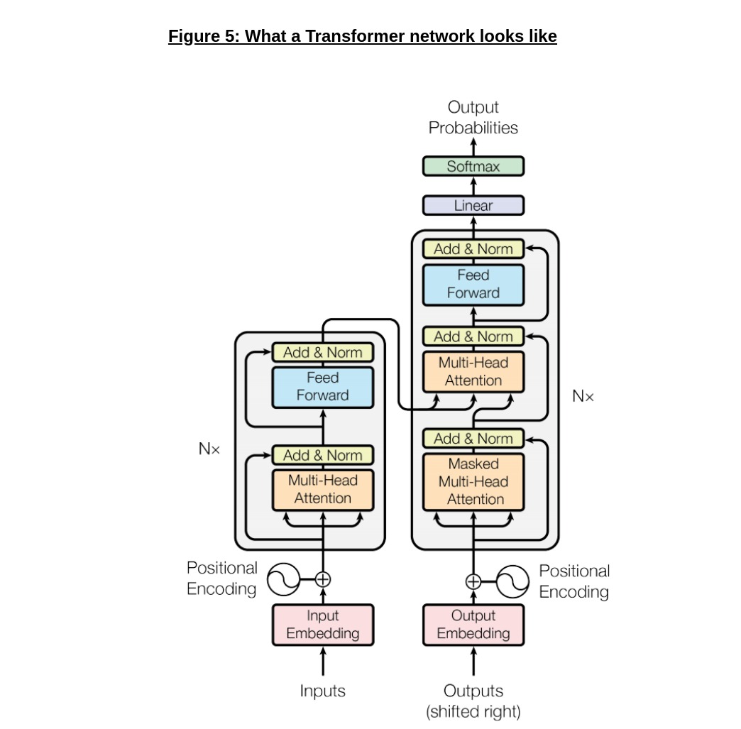
Above, in figure 5, we can see what a Transformer network actually looks like. We’ll break down each of the components in a minute, but I want to draw your attention (pun intended) to a few points first:

As promised, there is no recurrence in here whatsoever; the network uses attention directly at each layer to encode dependencies, and stacks multiple encoder (or decoder) layers to add representational power.
We also have skip connections around the attention and feed forward blocks, a idea that originates with ResNet and makes it easier to train the Transformer.
Already, we can start to see the increased scope for parallelism; feed-forward layers have no dependencies between input positions, and are ideal for acceleration (and GPU use)!

Input and Output Embeddings

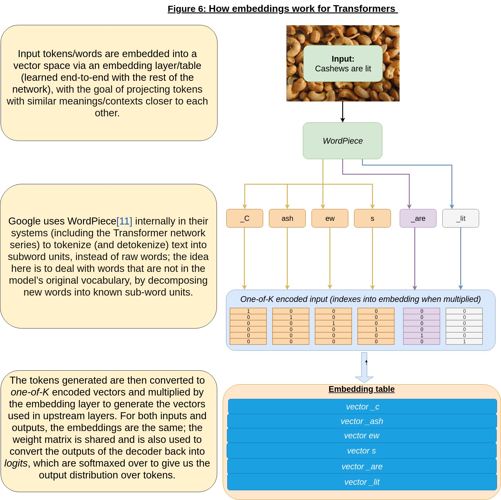
As seen in Figure 6, embeddings for Transformer networks are fairly standard, and are largely based on Google’s Neural Machine Translation System: Bridging the Gap between Human and Machine Translation work [11].

While I won’t spend too much time on how the “word pieces” (as shown in the example above) are generated and mapped to vectors (and back), I will mention a few points (if you’re interested in the subject, do look into some of the papers I cite here which go into further details of this aspect).

To come up with the most efficient set of “word pieces”, they use the Byte Pair Encoding algorithm, adapted for word segmentation using the same method as in “Neural Machine Translation of Rare Words with Subword Units” [12]; this works by iteratively merging the most common pair of “bytes” (in this case, n-grams) in a corpus into one “byte”/symbol, which is later used to encode and decode the input text.
Both the source and target languages (in the NMT case) use the same shared set of wordpieces, making it easier to directly copy rare words/numbers from the source to the target representation. As seen in the diagrams above, they also use some tricks, such as a special start of word symbol “_”, to help reverse the tokenization.
WordPiece itself is Google-internal only, but they have also released SentencePiece [13], a similar tokenizer/de-tokenizer that uses many of the same techniques; if you want to train your own model, that might be a good place to start.
As noted in the diagram, the input and output embedding layers are identical and share the same weight matrix, an idea developed by Press et al in 2017 [14].

Positional Encoding

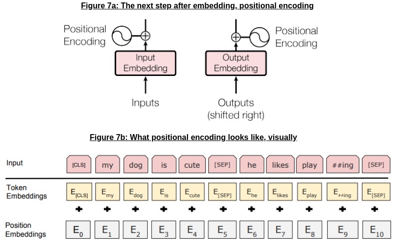
From Figure 7(a) above (a cropped version of the original architecture in Figure 5), the next step after the embedding stage (for both the encoder and decoder modules of the Transformer) is positional encoding. As we can in Figure 7(b), this adds information about the position of a token in an input sentence to the embedding we saw in the last section.

Why do we need this, though? The reason we need this in Transformers is the lack of recurrence: ordinary RNNs implicitly encode the position of a token in the hidden step at time \(t\) (which, we hope, has some memory of all the tokens it has seen before in time steps \([0, t-1]\)), but Transformer networks have no such “state”! The position of a word in a sentence is worth gold in NLP, and encoding that information directly is critical to helping the Transformer network compensate for the lack of recurrence.

As for what the encoding actually looks like, Fig 7(a) already hints at this; if you look at the icon for positional encoding, the shape inside it is - you guessed it - sinusoidal! (If the word is unfamiliar, it basically means sine/cosine-shaped curves).

Given an input token embedding in \(d_{model} = 512\) dimensions (for example), the positional encoding layer adds a sine-based encoding in even-numbered dimensions, and a cosine-based encoding in odd-number dimensions, represented by the formula below and shown in Figure 8:

\[PE_{(pos, 2i)} = sin(pos/10000^{(2i/d_{model})})\]
\[PE_{(pos, 2i+1)} = cos(pos/10000^{(2i/d_{model})})\]

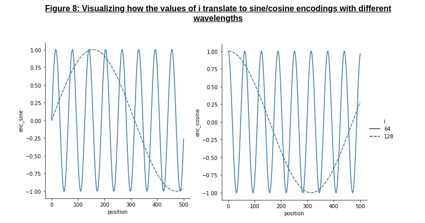
As we can see from the figure, this essentially involves a sine/cosine-based encoding with increasing wavelengths for higher dimensions, which gives the model different scales/signs for embedding the position for each token; Vaswani et al also experimented with other encoding mechanisms, and found that this worked the best.

Scaled Dot-Product Attention: the attention mechanism used in Transformers

Now we turn our attention (pun, once again, intended) to the attention mechanism used in Transformers - scaled dot-product attention. For this (and the next few sections), I will be borrowing a few graphics from Jay Alammar[15], who has done a fantastic job at visualizing how a Transformer network works (to the point that lectures at MIT have used his visualizations!).

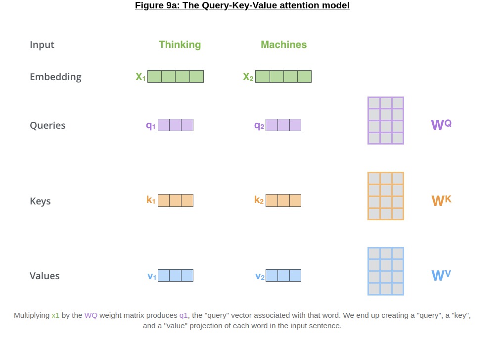
Transformer networks “transform” the input embedding for each token/part of the input (for stacked layers) into three parts - queries, keys and values. The queries, keys and values are all generated from each token, which allows the Transformer to perform self-attention (where the outputs are based on attending to different parts of itself).

The queries and keys model the interaction between different parts of the inputs
The values are generated by keeping in mind what information might be useful for the output (or for upstream layers), and are what we modify/blend via query-key dot products.

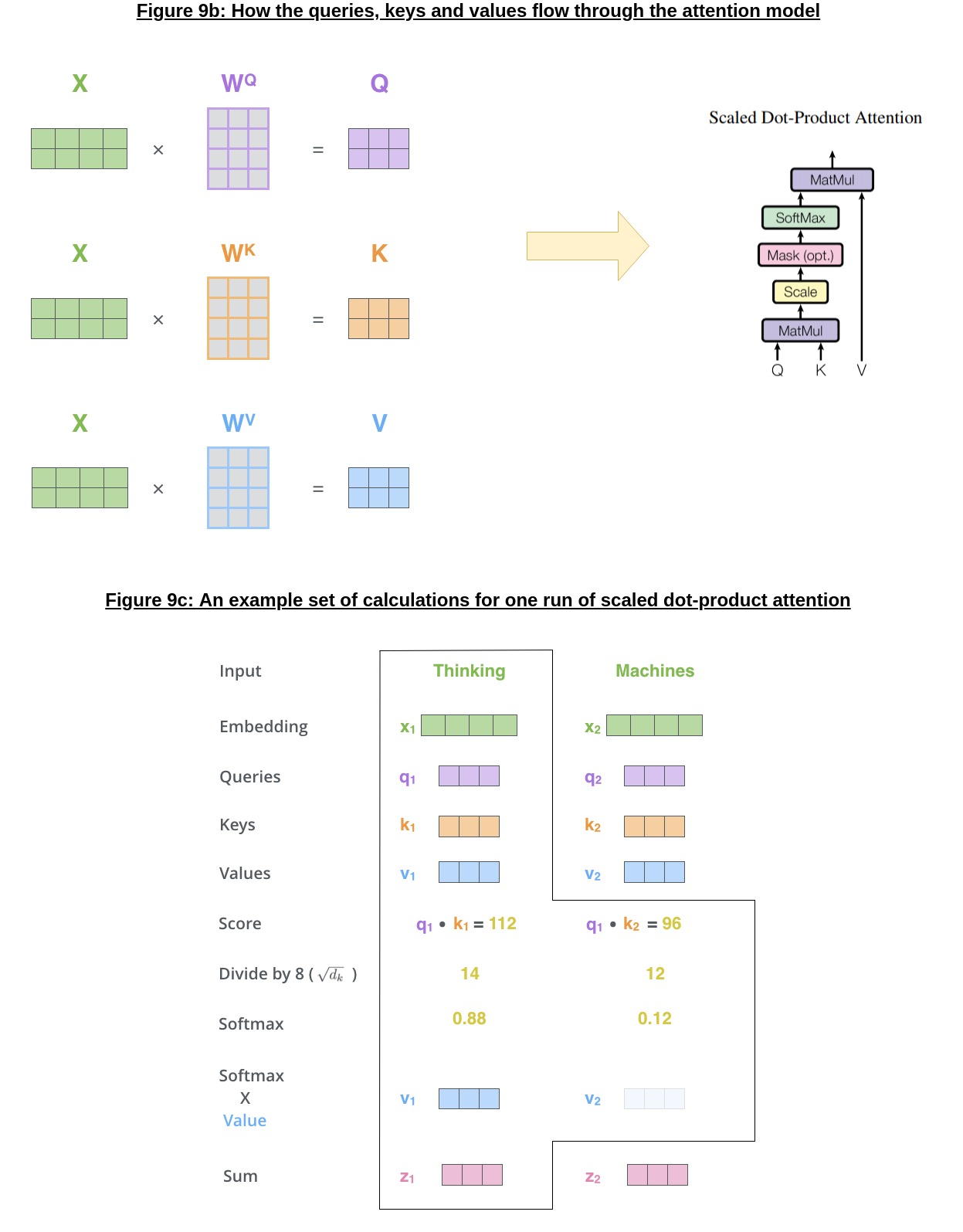As the transformations can get slightly long, I’ve used Figures 9b and 9c (above) to better demonstrate (as opposed to a wall of text) how the queries, keys and values are composed together into an entire scaled dot-product attention “layer”. The only points I will birefly make before going to the next section are:

\(W_{Q}, W_{K}, W_{V}\) are all learned through the course of training the network, and are applied to each set of input tokens separately (which ties back into the original motivation of parallelism in NLP!)
We “scale* down the output of the \(q_1^{T}k_{1}\) by \(\sqrt{d_k}\) to make the softmax gradients better behaved (if we were to softmax without rescaling, \(p_{112} = \dfrac{e^{112}}{e^{96} + e^{112}} \approx 1.0\))

Multi-Head Attention

As I’ve reiterated throughout this article, the entire motivation for going with an attention-only model has been to maximize parallelism, which brings us to the final component of the entire attention mechanism in Transformers - multi-head attention, as shown in Figure 10 below:

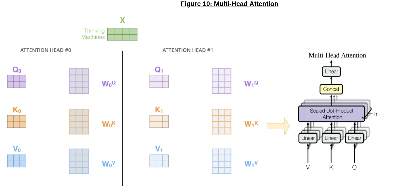
The idea is straightforward, but powerful; we can run multiple attention “heads” in parallel, and combine their outputs; this allows for much more parallelism, as each head can be computed separately, which is ideal for model parallelism (where different parts of the model are on different GPUs/nodes).

Bringing it all together!

Going back to Figure 5 (reposted below), we can now fill in the last few details, and take in the Transformer as a whole:

The outputs of the multi-head attention layers are followed by “Add & Norm” blocks; these simply add the inputs and outputs of the multi-head attention layers, and put them through a LayerNorm operation [16], an alternative to batch normalization developed for networks like RNNs or Transformers that have variable-length inputs (or test inputs that could be of different lengths).
The encoder is built out of stacked blocks using multi-head attention, add&norm and a standard two-layer feedforward network (with a ReLU activation) applied to each position independently
The decoder is almost the same, except for a few differences.
- The first part of a decoder block uses Masked Multi-Head Attention; this is the same as normal multi-head attention, except for the fact that, when taking the softmax of query-key products, we zero out keys who correspond to positions after the input used for a query. This makes sure that say, while deciding what to output at time step \(t\), we don’t factor in any interaction between the queries for \(t = 0\) and keys at \(t - 1\), since the output at \(t = 0\) cannot “attend” to outputs after itself.
- After the Masked multi-head and add&norm, we have a standard multi-head attention block with one, crucial twist - the keys and values come from the final block of the encoder, while only the queries come from the downstream layer! This allows the decoder at each time step to attend to all parts of the input, in addition to whatever it has outputed so far. Note that this applies for each decoder block, as shown in the animation below:

How is the Transformer trained and tested?

Importantly, the Transformer network is trained in the same way as any standard sequence-to-sequence RNN, as a supervised (this, despite seeming obvious, becomes much more important when we get to GPT and BERT) network, using a dataset of English-German or English-French sentences.

Our loss function is the negative log probability of a correct translation T given a source sentence S, over the entire dataset \(S\), as shown below:

\[L(W) = \frac{1}{S} \sum_{(T, S \in S)} - \log p_{W}(T|S)\] \[p_{W}(T|S) = \prod_{y_i \in S} p_{W}(y_{i} | y_{i-1}, y_{i-2} ... )\]

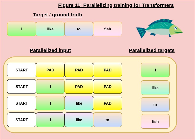
When training, we use teacher-forcing; regardless of the output of the decoder at \(T = t\), we feed in the ground-truth tokens as our decoder input for \(T = t + 1\); this prevents the model’s errors at \(t\) propogating further in its decoded output for \(t + 1\) and further while training, and makes it much easier to train the model.
Importantly, because we know the ground-truth labels while training, we can actually parallelize the training for a sequence very effectively by batching together all the possible “partial translations” and corresponding targets together, as shown in Figure 11 below [17]:

Note that this trick can’t be used with RNNs - an RNN needs to compute the state at each time step before taking in the next input, making it incapable of using such a method to train well; this shows us how the Transformer harnesses parallelism much more efficiently!
When testing, we simply sample the most likely output by taking the last element of the final softmax at each (or, in the case of beam search, the k-most likely outputs of the last position) at each time step, and add it to our current partial translation ((s), if using beam search to maintain a a list of k-most likely partials), which is fed into the decoder at each time step.

For more details on the hyperparameter, GPU and dataset configurations, feel free to check out the original paper[2] - I focused more on the idea-level for each component, but if you’re looking to use it on your own dataset, the original paper is the best place to start.

Impact

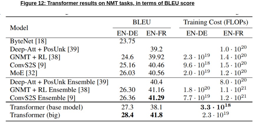
This will become more fleshed out in the next post (when we look at direct descendants of the Transformer), but suffice to say that the Transformer network was absolutely revolutionary! It was:

The first time we had a fully attention-based network, instead of a recurrent-plus-attention model
It established itself as state-of-the-art on machine translation tasks (as shown in the table below), while also requiring less FLOPS (Floating Point Operations) to train to this state-of-the-art parameter setting
Gave rise to a medley of Transformer-based architectures, some of which we will go through in the next post!

Citations

[1] High Voltage Feed Windstrom: Erich Westendarp, Pixabay
[2] Attention is all you need: Vaswani et al, 2017
[3] Improving Language Understanding by Generative Pre-Training: Radford et al, 2018
[4] Language Models are Unsupervised Multitask Learners: Radford et al, 2019
[5] BERT: Pre-training of Deep Bidirectional Transformers for Language Understanding: Devlin et al, 2019
[6] CS 231n, Lecture 10: Profs. Fei-Fei Li, Justin Johnson and Serena Yeung, Stanford University, 2017
[7] Sequence to Sequence Learning with Neural Networks: Sutskever et al, 2014
[8] Peeking into the neural network architecture used for Google’s Neural Machine Translation: Stephen Merrity, 2016
[9] A robin: Oldiefan, Pixabay
[10] Neural Machine Translation by Learning to Jointly Align and Translate: Bahdanau et al, 2016
[11] Google’s Neural Machine Translation System: Bridging the Gap between Human and Machine Translation: Wu et al, 2016
[12] Neural Machine Translation of Rare Words with Subword Units: Sennrich et al, 2016
[13] SentencePiece: Google
[14] Using the Output Embedding to Improve Language Models: Press et al, 2017
[15] Illustrated Transformer: Jay Alammar
[16] Layer Normalization: Ba et al, 2016
[17] Fish Sea Water Swim: kreatikar, Pixabay