Automating ML: Neural Architecture Search

Introduction
Some of you might have seen or heard about Google Cloud’s recent AutoML offerings (starting with AutoML for Vision last year). As shown below [2], the service offers ML-as-a-service in a sense by handling model design, training and deployment for you automatically, and has been a big hit with companies who want to use ML but lack the expertise.
![[2]](https://miro.medium.com/max/680/1*Obignp0mKyVuHx07XZhgGQ.gif)

But how does it work? AutoML involves a lot of techniques, but one of the most important of them is NAS(Neural Architecture Search), the subject of today’s post - an area of research that investigates how we can automate neural network design.
Using the following key papers in the field as a reference, we’re going to dive into NAS and explore how it actually works:
-
Neural Architecture Search with Reinforcement Learning [3]
-
Efficient Neural Architecture Search via Parameter Sharing [4]
-
DARTS: Differentiable Architecture Search [5]
Because this series is a bit more explorative, we won’t be going much into the actual results of the papers (what their accuracies were on CIFAR10 for convolutional nets or Penn Treebank for recurrent nets); the focus here is on the core ideas, and while I will allude briefly to how methods perform, the papers are linked throughout the article and in the bibliography, so definitely look into those for the nitty-gritties of performance.
NAS with RL
Core idea
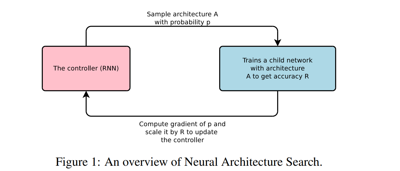
Figure 1 (above) shows us the fundamental idea of the paper Neural Architecture Search with Reinforcement Learning, published by Barret Zoph and Quoc V. Le at Google Brain in 2017.
The first key point the authors make is this: the structure and connectivity of a neural network, like many other things, can be represented as a variable length string; you can decompose each layer into its design parameters (number of filters, filter dimensions, stride in each dimension, etc), and represent the network as a concatenation of those parameters, layer-by-layer.
What that also means, however, is that you can have a recurrent neural network “generate” such a string; by discretizing those parameters and constraining them (for example, by restricting filter height \(\in [3, 5, 7]\)), we can have an RNN generate an architecture by softmaxing over the distribution of parameters at each step, as shown below in Figure 2 (from the original paper):
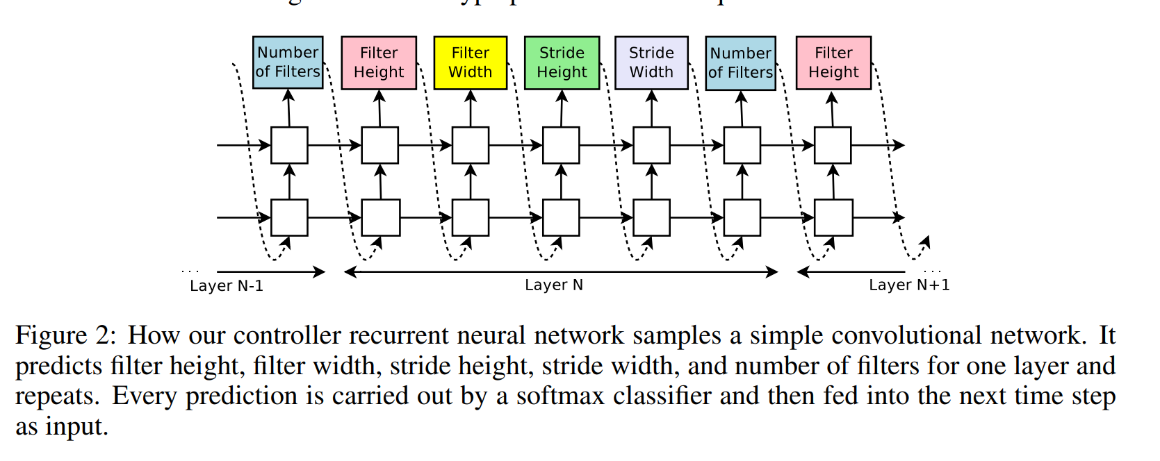
Using this process, we can generate an architecture, train it and use the accuracy as a guideline for choosing future architectures!
Unfortunately, however, this does involve some complexity; if the parameters of your RNN controller are \(\theta_{c}\), and the loss of your child network \(A\) is \(L(y, f_{\theta_{A}}(x))\), there’s no direct way to compute the gradient of that loss with respect to \(\theta_{c}\). You can differentiate the loss with respect to \(\theta_{A}\), but converting that into a signal for the design decisions of controller network requires the REINFORCE trick from reinforcement learning.
How REINFORCE is used to train NAS
REINFORCE is a method used in reinforcement learning to train decision-making networks (like the RNN controller in NAS), using a set of log-based transformations and probability tricks to derive a policy gradient for the “reward” we saw at each training iteration. If you want to learn more about the method, I highly encourage you to go over these slides from Prof. Sergey Levine’s class on Deep RL.
When applying REINFORCE to NAS, it turns out the NAS setup is actually a little simpler:
-
Unlike standard RL (where you get some reward at each step), there is only one reward at the very end of the designing process - the validation accuracy of the trained child network.
-
The transition function is completely deterministic - given a current state and an “action”/decision, there is no stochasticity in the next state, so we can drop the “states” and only optimize over actions (you can always reconstruct the states from a set of actions)
This reduces our objective to:
\[J(\theta_{c}) = E_{p(a_{1:T}; \theta_{c})} [R]\]Where \(R\) is the validation accuracy of the subsequent model we train; applying the policy gradient method to this yields the following gradient:
\[\nabla_{\theta_{c}} J(\theta_{c}) = \sum_{t=1}^{T} E_{p(a_{1:T}; \theta_{c})} [\nabla_{\theta_{c}} \log P(a_{t} | a_{t-1: 1}; \theta_{c}) R]\]In practice, the authors reduce the variance of the policy gradient by using a common trick, subtracting a baseline (in this case, an exponential moving average of previous architecture accuracies), which makes our gradient as follows:
\[\nabla_{\theta_{c}} J(\theta_{c}) = \frac{1}{m} \sum_{k=1}^{m} \sum_{t=1}^{T} E_{p(a_{1:T}; \theta_{c})} [\nabla_{\theta_{c}} \log P(a_{t} | a_{t-1: 1}; \theta_{c}) (R_k - b)]\]Where \(m\) is the “batch size” of architectures we generate in parallel, and \(b\) is the baseline.
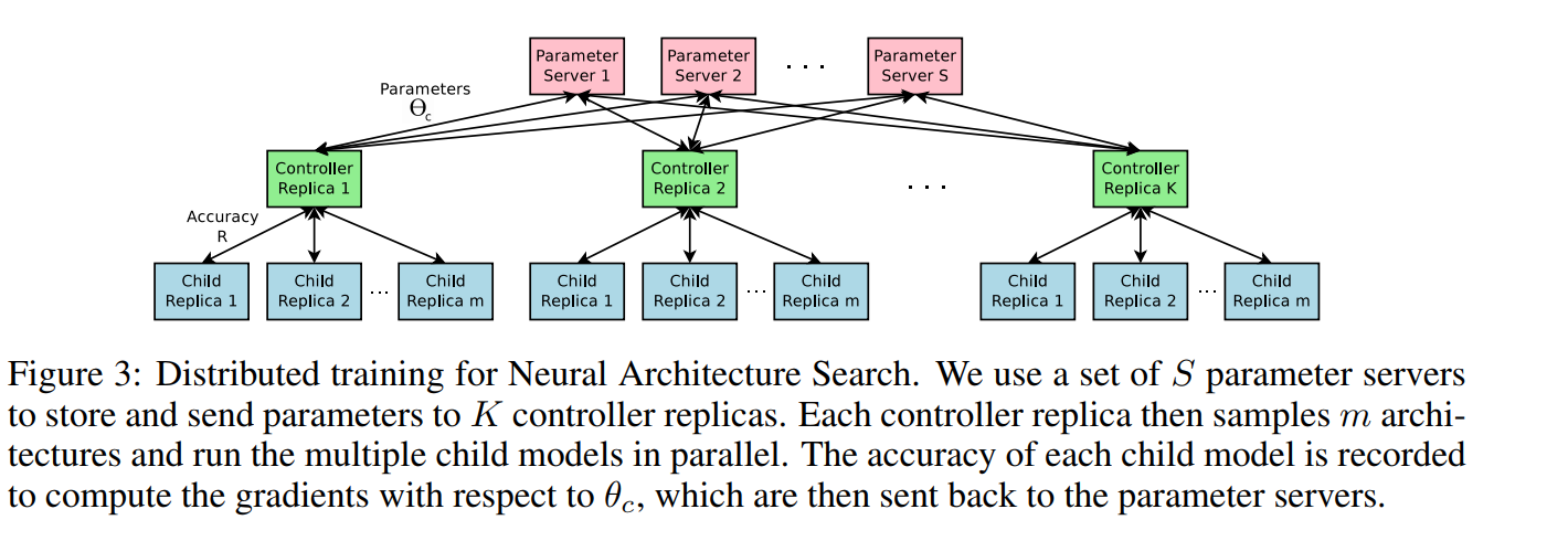
As you might suspect, however, this process can be very lengthy - you need to train a batch of \(m\) child networks at each step, then synchronize the policy gradient from each into the controller RNN. To speed this up, the authors of NAS with RL used a specializied distributed training setup, as shown in Figure 3 below:
Skip connections
While the NAS framework, as currently outlined, would work well for generating basic CNNs, skip connections are another key component of most modern CNN architectures; introduced by the ResNet paper in 2015 [7], these help us develop much deeper networks by alleviating some of the issues with optimizing deeper nets.
In order to fit skip connections into the NAS framework, the authors added a new type of decision/state at each layer - an anchor point. As shown in Figure 4 below, the anchor point is added before the start of each layer, and can connect to each of the previous layers - a decision the RNN controller makes for each anchor point.
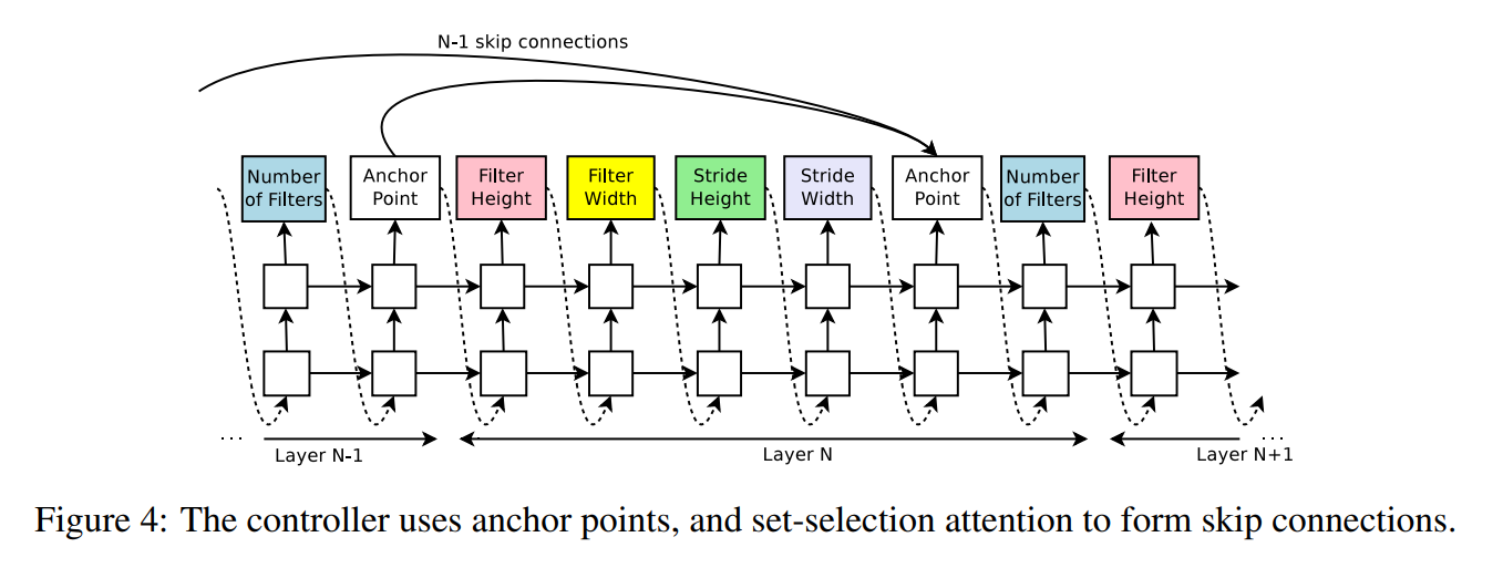
To make the decision for what layers to connect to the current layer, the authors parametrize the probability below:
\[P(\text{Layer j is an input to layer i}) = \text{sigmoid}(v^{T}\text{tanh}(W_{prev}*h_{j} + W_{curr}*h_{i}))\](Where \(h_{j}\) is the hidden state of the RNN controller at the anchor point for layer \(j\), and \(W_{prev}, W_{curr}, v\) are learned parameters.)
At each anchor point, the RNN controller samples from this distribution for all previous layers, and uses the sampled outputs to connect different layers (using padding to account for differences in layer sizes).
RNN cells
As we’ve seen above in the last few sections, the NAS with RL method can generate CNN architectures (with multiple skip connections) - but can it also be extended to RNNs?
To do this, the authors decided to focus on one cell of an RNN; the structure that, given a previous hidden state \(h_{t-1}\) and input \(x_{t}\), produces a new hidden state \(h_{t}\) that is used for output or as input to upstream layers.
The vanilla RNN, for instance, has \(h_{t} = \text{tanh}(W_{xh}*x_t + W_{hh}h_{t-1})\); the more widely used cell, the LSTM, also has a cell variable (\(c_{t-1}, c_{t}\)) to represent memory states.
As shown in Figure 5 below, NAS can be adapted to generate such a cell by developing a computational tree that maps (\(h_{t-1}, c_{t-1}, x_{t}\) to \(h_{t}, c_{t}\)).
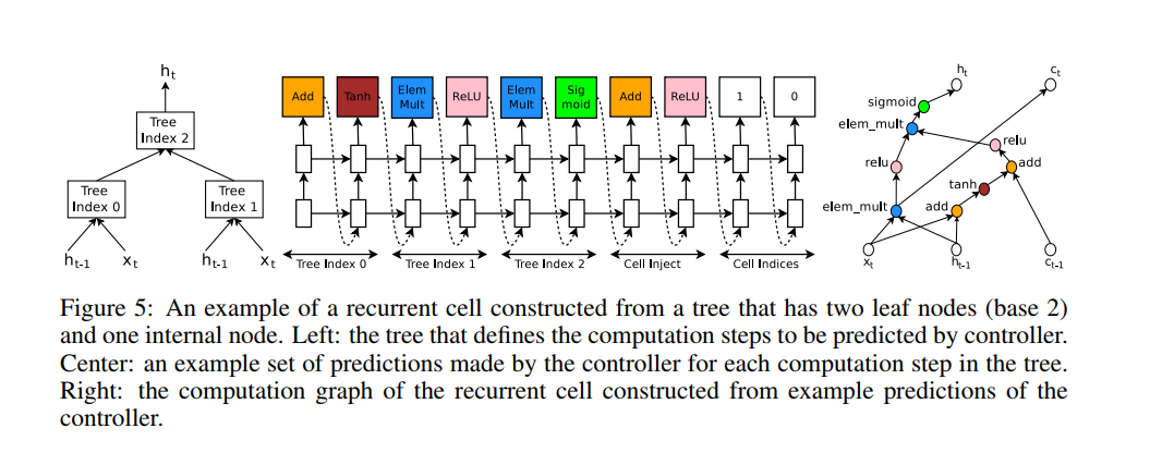
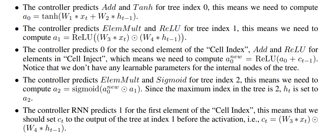
At each index, the RNN generates two operations - a combiner (addition, elementwise multiplication, etc) and an activation (Tanh, ReLU, Sigmoid, etc), which are applied to combine the two inputs to the index (with weight matrices applied while combining); as we can see in the diagram, the first few indices are combinations of \(h_{t-1}, x_{t}\), while higher level tree nodes combine these to generate \(h_{t}\). The cell injects/indices steps do something similar, but for \(c_{t-1} \rightarrow c_{t}\).
Since this might be a bit dense without an example, the authors have also provided a step-by-step walkthrough of the steps in Figure 5, which I’ve pasted below:
Recap: NAS with RL
I’m going to repaste Figure 1 below again to provide a quick recap of what we’ve seen of NAS with RL so far:
RL with NAS:
-
Uses an RNN controller to make design decisions at each step; for CNNs, this is the filter dimensions, stride in each dimensions, skip connections, etc, while for RNNs the controller designs it at a more cellular level (the cells are then used to build a child network).
-
While training, samples architectures from the RNN (using the probability distribution of the output at each time step), and uses REINFORCE to update the controller parameters using the performance of the child networks.
ENAS: Efficient NAS
The first approach we saw, NAS with RL, was a good starting point in terms of generating new architectures/cells; however, it was also incredibly inefficient!
-
It took ~450 GPUs for 3-4 days \(\rightarrow\) 30k+ GPU hours to train NAS and obtain state-of-the-art results!
-
Using RL-based approaches with less compute time (as in [8], which used a Q-Learning approach) led to good but not as strong results/networks.
Why is this process so inefficient? The biggest problem as correctly idenfitied by the authors of ENAS is the fact that, for each child network, we train an entire model and find the validation accuracy but throw the trained parameters away!
In order to solve this problem and speed up the NAS process, the authors of ENAS propose a remarkable solution - weight-sharing, shown below in Figure 6:
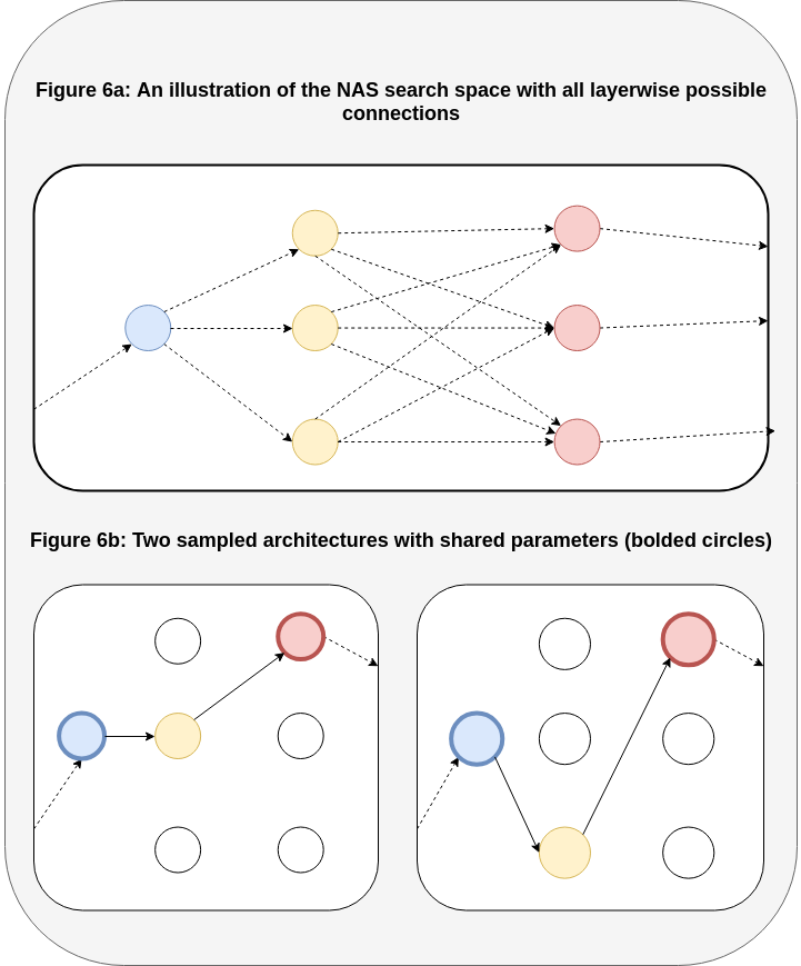
Figure 6a shows us NAS at a higher, layerwise node level (instead of each specific decision); at each set of steps we have a range of possible layers to choose from, with each complete network represented as a path in the supergraph.
In the NAS with RL approach, we would select a path of nodes in the supergraph and train the parameters for those nodes from scratch; what ENAS proposes, as shown in Figure 6b, is to retain the weights from previous choices, and share them across all child models in the search space! With the ENAS approach, we:
-
Sample a path of nodes in the supergraph to form a child network (via an RNN controller)
-
Continue training the parameters of those nodes, and update them, via some variant of SGD with respect to the loss (e.g. cross-entropy), in both the current model and the supergraph!
-
Use the performance of the models sampled by the controller to train the controller (via REINFORCE or other means).
The upside of this approach is massive; the sharing of weights (via the supergraph) allows us to get much more work out of the training of child networks (as opposed to just one number, the validation accuracy), and shares the benefits throughout the process.
To make this approach work, here are some practical details:
-
Search space: ENAS restricts the search space by compressing the per-attribute decisions (e.g. stride, filter height, width) into deciding from sets of pre-defined attributes (e.g. 5x5 convolutions, 3x3 depthwise-separable convolutions, 3x3 average pooling).
-
Training: ENAS also alternates training of the shared weights \(\omega\) and the controller \(\Theta\) by phases; the supergraph weights are trained by SGD, while the LSTM controller is trained with Adam + REINFORCE
-
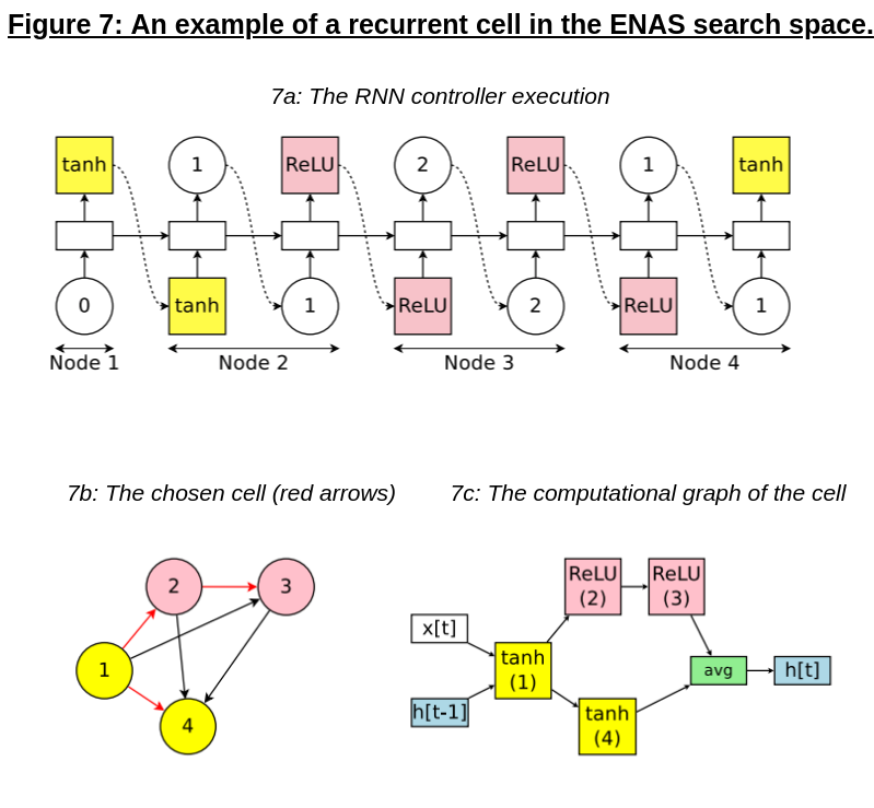
ENAS for cells: As shown in Figure 7 below, ENAS can also be used to generate cells and cellular-based architectures; unlike the NAS with RL approach, the topology of cells is not limited to trees, and extends to general computational graphs (any nodes with no outward edges at the end of cell design are averaged together and used as the cell output)
-
Results: While we won’t discuss results much in this article, it’s important to note that the ENAS approach is 1000x faster than the NAS with RL approach, needing only around 8 GPU hours to find a near state-of-the-art architecture on CIFAR10
DARTS: Differentiable NAS
Going from discrete to continuous
While ENAS was a huge improvement on NAS with RL, it still suffers from some of the same problems, albeit on a smaller scale, as do other approaches. Specifically, the NAS problem as currently framed is an optimization problem in a discrete search space - each potential architecture arises from a discrete set of design decisions, which makes the architecture search space exponential in size and hard to optimize in.
A common trick from optimization when faced with discrete problems is to relax the discrete constraints into continuous ones and optimize over the continuous problem; after you solve the continuous problem, you can recover a discrete solution, which is often optimal or at least good for the original problem. But can this be applied to NAS?
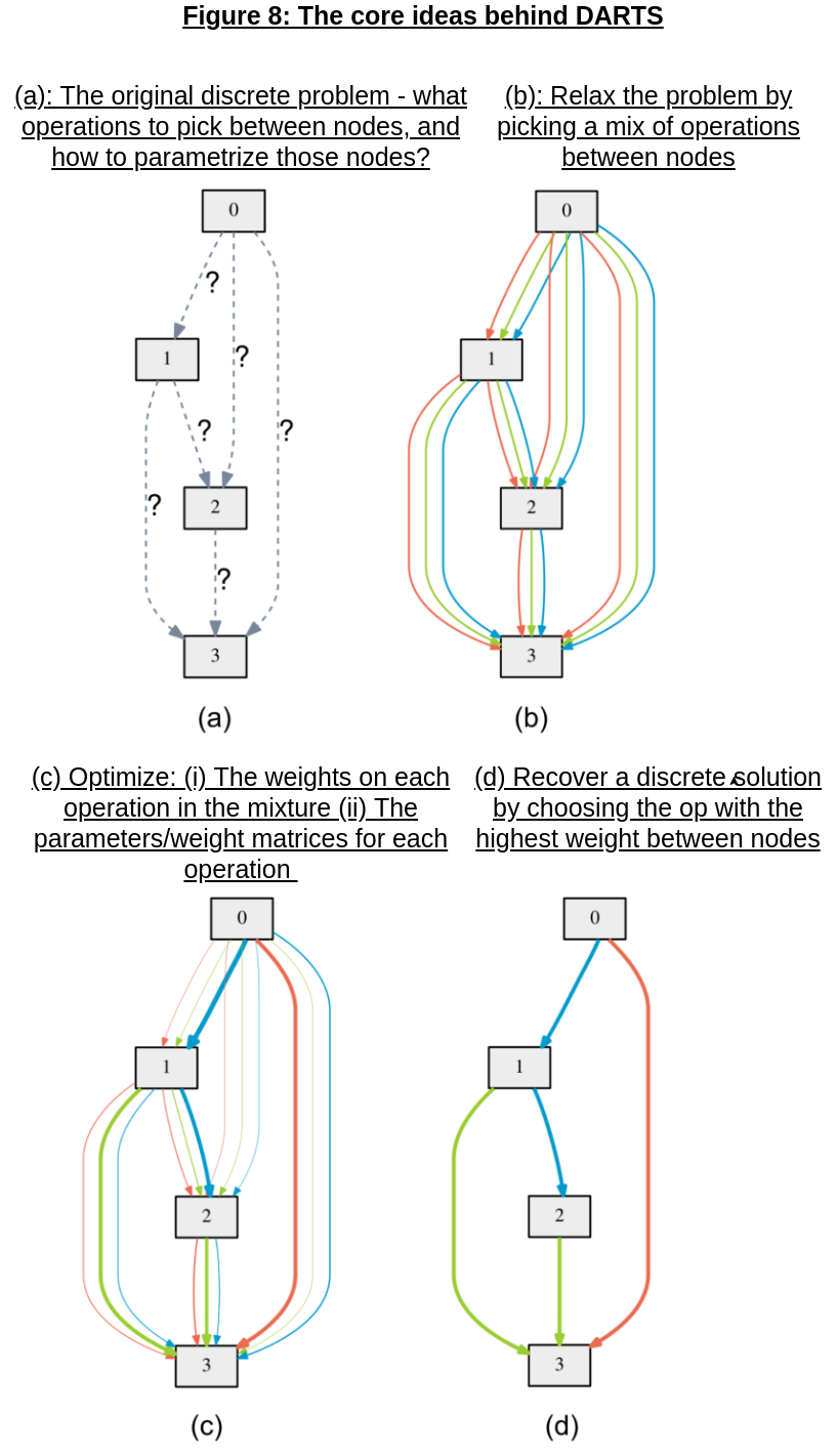 That’s where DARTS comes in! As shown in Figure 8 above, DARTS operates on a cellular level, searching for convolutional/recurrent cells that are stacked together to form the generated architecture. The method works by relaxing the “discrete set of operations” optimization problem into a “continuous mixture of operations” problem, and discretizes the continuous solution by picking the operation between each node with the maximum weight.
The advantages of this approach are that it is:
-
Directly differentiable: Now that the problem is continuous, you can apply your favorite optimizer (with some mathematical tricks, as we will see soon) and differentiate the objective directly! You no longer need to use methods like REINFORCE/RL or evolutionary strategies, as the DARTS formulation is now in the framework of well-known optimization problems.
-
Controller-free: Another benefit of the DARTS formulation is that we are now simply optimizing over two set of weights (node weights and operation weights) - we no longer need a controller to generate the architecture of the network/cell at each step, as we can simply solve the continuous problem and discretize to “generate” an architecture.
-
Results-wise: The method outperforms previous methods like NAS with RL while being orders of magnitude lower in computational cost; while the method is a bit more expensive than ENAS, the cells DARTS generates are also slightly better than ENAS. There’s also a github repository associated with the paper here, so definitely check it out and play around with it!
The mathematics behind DARTS
While the idea itself is fairly simple, it does require some clever math to formulate and solve the problem efficiently.
The original, discrete cell formulation looks something like this: for a given cell with N nodes, each intermediate node \(x^{(j)} = \sum_{(i < j)}o^{(i, j)} (x^{(i)})\), where \(o^{(i, j)}\) represents a chosen operation on \(x^{(i)}\) (e.g. convolution, scalar multiplication, or the zero operation to indicate a lack of connection between nodes).
We first relax \(o^{(i, j)}\) continuously as the softmax over all operations (weighted):
\[\bar{o}^{(i, j)}(x) = \sum_{o \in O} \dfrac{exp(a_o^{(i, j)})}{\sum_{o' \in O} exp(a_{o'}^{(i, j)})} o(x)\]Searching for cell architectures now translates to learning \(a = a_{o}^{(i, j)}\), the weights on each operation between intermediate nodes \((i, j)\); given this, we can formulate the overall problem as:
\[\min_{a} \text{L}_{\text{val}}(w^{*}(a), a) \\ \text{s.t. } w^{*}(a) = \text{argmin}_{w} \text{ L}_{\text{train}} (w, a)\]\(\text{L}_{\text{val}}, \text{ L}_{\text{train}}\) represent the validation and training losses respectively; this is termed as a bilevel optimization problem (as it involves two levels of optimization), and also arises in other forms of AutoML like gradient-based hyperparameter optimization [9].
Solving this kind of nested problem can be very computationally expensive, but it can be approximated with a simple idea - while optimizing \(a\), we can replace \(\nabla_{a} \text{L}_{val}(w^{*}(a), a)\) with:
\[\nabla_{a} \text{L}_{\text{val}}(w - \xi \nabla_{w} \text{L}_{\text{train}}(w, a), a)\]The key difference is that we don’t solve the inner optimization completely by training to convergence; instead, we adapt \(w\) with a single training step. While there are no convergence guarantees with this modification, the approximation seems to reach a fixed point on \(a\) in practice (as we take more steps, the weights get closer and closer to \(w*\)). Given this approximation, the DARTS algorithm looks as below:
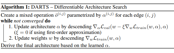
There is one more key point to make here - what does \(\nabla_{a} \text{L}_{\text{val}}(w - \xi \nabla_{w} \text{L}_{\text{train}}(w, a), a)\) looks like?
If we apply the chain rule to the expression and let \(w' = (w - \xi \nabla_{w} \text{L}_{\text{train}}(w, a)\), we get:
\[\nabla_{a}L_{val} (w', a) - (\nabla_{w'}L_{val}(w', a)) (\xi \nabla_{a, w}^{2} L_{train}(w, a))\]In practice, the authors evaluate the second term via a finite-difference approximation; letting \(\epsilon\) be a small scalar, and \(w^{\pm} = w \pm \epsilon \nabla_{w'}L_{val}(w', a)\), we can approximate the second term as:
\[\approx \dfrac{\nabla_{a}L_{train}(w^{+}, a) - \nabla_{a}L_{train}(w^{-}, a)}{2\epsilon}\]Recap, and further reading
To briefly recap what we’ve seen of NAS today:
-
NAS with RL was one of the first papers about NAS; it used a RNN controller to generate networks by making layerwise/cellular design choices, and used REINFORCE to train the controller
-
ENAS: Efficient NAS made the above approach a lot more efficient by treating each choice/operation as a node of parameters in a supergraph and forcing common nodes between architectures to share parameter weights.
-
DARTS: Differentiable Architecture Search removed the need for the controller+RL/evolution strategy by defining NAS in a differentiable way, allowing you to train the design choice weights directly with gradient descent
If you thought the ideas in these papers were cool and want to learn more about NAS and current work in the field, check out this literature list - it contains a huge number of papers in NAS, of which the bolded ones were accepted at conferences.
Citations
- [1] Automation Memes
- [2] How does Cloud AutoML work: Original source
- [3] Neural Architecture Search with Reinforcement Learning: Zoph et al, 2017
- [4] Efficient Neural Architecture Search via Parameter Sharing: Pham et al, 2018
- [5] DARTS: Differentiable Architecture Search: Liu et al, 2019
- [6] CS 294-112 Fall 2017, Lecture 4: Levine et al, 2017
- [7] Deep Residual Learning for Image Recognition: He et al, 2015
- [8] Designing Neural Network Architectures Using Reinforcement Learning: Baker et al, 2017
- [9] Gradient-based Hyperparameter Optimization through Reversible Learning: Maclaurin et al, 2015
![[1]](https://i.imgflip.com/1l1t5h.jpg)